12. The Inca - Cities in the Cloud (Part 2 of 2)

Randall Carlson Podcast Ep032 St-Jean & Nipigon Impacts? Problematic Ene...

Randall Carlson Podcast Ep029 Fingerprints of Catastrophe / Range of Imp...

No Such Thing as a Free Lunch: Principles of Economics (Part 138)

That's the world we live in: when it comes to economics, people have emotions; it's not like chemistry or physics.

Robert J. Shiller

Aggregate Demand, Aggregate Supply, and Inflation

(Part G)

by

Charles Lamson

Aggregate Demand, Aggregate Supply, and Monetary and Fiscal Policy

FIGURE 11

Figures 11 and 12 show that it is important to know where the economy is before a policy change is put into effect. The economy is producing on the nearly flat part of the AS curve if most firms are producing well below capacity. When this is the case, firms will respond to an increase in demand by increasing output much more than they increase prices. If the economy is producing on the steep part of the AS curve, firms are close to capacity and will respond to an increase in demand by increasing prices much more then they increase output.

To see what happens when the economy is on the steep part of the AS curve, consider the effects of an increase in G with no change in the money supply. What will happen is that when G is increased, there will be virtually no increase in Y. In other words, the expansionary fiscal policy will fail to stimulate the economy.

The first thing that happens when G increases is an unanticipated decline in the firm's inventories. Because firms are very close to capacity output when the economy is on the steep part of the AS curve, they cannot increase their output very much. The result, as Figure 12 shows, is a substantial increase in the price level. The increase in the price level increases the demand for money, which (with a fixed money supply) leads to an increase in the interest rate, decreasing planned investment. There is nearly complete crowding out (phenomenon that occurs when increased government involvement in a sector of the market economy substantially affects the remainder of the market, either on the demand or supply side of the market) of investment. If firms are producing at capacity, prices and interest rates will continue to rise until the increase in G is completely matched by a decrease in planned investment and there is complete crowding out.

Long-Run Aggregate Supply and Policy Effects

We have so far been considering monetary policy and fiscal policy effects in the short run. Concerning the long run, it is important to realize:

The AS curve is vertical in the long run, neither monetary policy nor fiscal policy has any effect on aggregate output in the long run.

The conclusion that policy has no effect on aggregate output in the long run is perhaps startling. Do most economists agree that the aggregate supply curve is vertical in the long run? 

Most economists agree that input prices tend to lag behind output prices in the short run, giving the AS curve some positive slope. Most also agree that the AS curve is likely to be steeper in the long run, but how long is the long run? The lower the lag time, the greater the potential impact of monetary and fiscal policy on aggregate output. If the long run is only three to six months, policy has little chance to affect output; if the long run is 3 or 4 years, policy can have significant effects. A good deal of research in macroeconomics focuses on the length of time lags between input and output prices. In a sense, the length of the long run is one of the most important open questions in macroeconomics.

The "new classical" economics assumes prices and wages are fully flexible and adjust very quickly to changing conditions. New classical economists believe, for example, that wage rate changes do not lag behind price changes. The new classical view is consistent with the existence of a vertical AS curve, even in the short run. At the other end of the spectrum is what is sometimes called the simple "Keynesian" view of aggregate supply. Those who hold this view believe there is a kink in the AS curve at capacity output.

*CASE & FAIR, 2004, PRINCIPLES OF ECONOMICS, 7TH ED., PP. 546-549*

end

741 Hz ❯ Spiritual Detox ❯ Remove Toxins & Negative Thoughts ❯ Mandala M...

No Such Thing as a Free Lunch: Principles of Economics (Part 137)

Economics, politics, and personalities are often inseparable.

Charles Edison

Aggregate Demand, Aggregate Supply, and Inflation

(Part F)

by

Charles Lamson

The Equilibrium Price Level

Figure 9 looks simple, but it is a powerful device for analyzing a number of macroeconomic questions. Consider first what is true at the intersection of the AS and AD curves. Each point on the AD curve corresponds to equilibrium in both the goods market and the money market. Each point on the AS curve represents the price/output responses of all the firms in the economy. This means:

The point at which the AS and AD curves intersect corresponds to equilibrium in the goods and money markets and to a set of price/output decisions on the part of all the firms in the economy.

 We will use this AS/AD framework to analyze the effects of monetary and fiscal policy on the economy and to analyze the causes of inflation. First we need to return to the AS curve and discuss its shape in the long run.

The Long-Run Aggregate Supply Curve

For the AS curve not to be vertical, some costs must lag behind increases in the overall price level. If all prices (both input and output prices) change at the same rate, the level of aggregate output does not change. We have assumed that in the short run at least some cost changes lag behind price level changes, but what happens in the long run?

Many economists believe costs lag behind price level changes in the short run but ultimately move with the overall price level. For example, wage rates tend to move very closely with the price level over time. If the price level increases at a steady rate, inflation may come to be fully anticipated and built into most labor contracts.

If wage rates and other costs fully adjust to changes in prices in the long run, then the long-run AS curve is vertical.

Potential GDP

Recall that even the short-run AS curve becomes vertical at some particular level of output. The vertical portion of the short-run curve exists because there are physical limits to the amount that an economy can produce in any given time period. At the physical limit, all plants are operating around the clock, many workers are on overtime, and there is no cyclical unemployment.

*CASE & FAIR, 2004, PRINCIPLES OF ECONOMICS, 7TH ED., PP. 544-546*

end

12. The Inca - Cities in the Cloud (Part 1 of 2)

No Such Thing as a Free Lunch: Principles of Economics (Part 136)

I don't go to the beach. There is no value in going to the beach. If I did go I would probably read economics books.

Esther Duflo

Aggregate Demand, Aggregate Supply, and Inflation

(Part E)

by

Charles Lamson

Shifts of the Short-Run Aggregate Supply Curve

Just as the aggregate demand curve can shift (See part 133), so to can the aggregate supply (price/outlet response) curve. Recall the individual firm behavior we just considered in part 135 in describing the shape of the short-run curve. Firms with the power to set prices choose the price/output combinations that maximize their profits. Firms in perfectly competitive industries choose the quantities of output to supply at given price levels. The AS curve traces out those price/output responses to economic conditions.

Anything that affects these individual firm decisions can shift the AS curve. Some of these factors include cost shocks, economic growth, stagnation, public policy, and natural disasters.

Cost Shocks Firms decisions are heavily influenced by costs. Some costs change at the same time the overall price level changes, some costs lag behind changes in the price level, and some may not change at all. Changes in costs that occur at the same time that the price level changes are built into the shape of the short-run AS curve. For example, when the price level rises, wage rates might rise by half as much in the short run. (This could happen if half of all wage contracts in the economy had cost-of-living increase clauses and half did not.) The shape of the short-run AS curve would reflect the response.

Sometimes cost changes occur that are not the result of changes in the overall price level---for example, the cost of energy. During the fall of 1990, world crude oil prices doubled from about $20 to $40 a barrel. Once it became clear the Persian Gulf War would not lead to the destruction of the Saudi Arabian oil fields, the price of crude oil on world markets fell back to below $20 per barrel. In contrast, in 1973 to 1974 and again in 1979, the prices of oil increased substantially and remained at a higher level. Oil is an important input in many firms and industries, and when the price of a firm's inputs rises, Firms respond by raising prices and lowering output. At the aggregate level, this means an increase in the price of oil (or a similar cost increase) shifts the AS curve to the left, as in Figure 7(a). A leftward shift of the AS curve means a higher price level for a given level of output.

FIGURE 7 Shifts of the Aggregate Supply Curve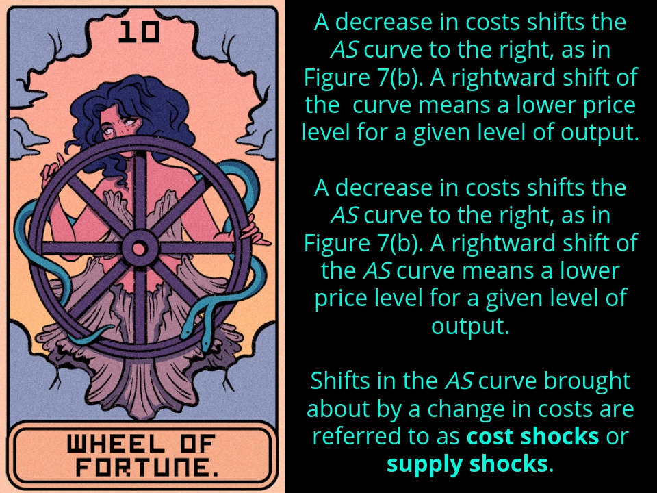

Economic Growth Economic growth shifts the AS curve to the right. Recall that the vertical part of the short-run AS curve represents the economy's maximum (capacity) output. This maximum output is determined by the economy's existing resources and the current state of technology. If the supply of labor increases or the stock of capital grows, the AS curve will shift to the right. The labor force is expected to grow naturally with an increase in working-age population, but it can also increase for other reasons. Since the 1960s, for example, the percentage of women in the labor force has grown sharply. This increase in the supply of women workers has shifted the AS curve to the right. 

Immigration can also shift the AS curve. During the 1970s, Germany, faced with a serious labor shortage, opened its borders to large numbers of "guest workers," largely from Turkey. The United States has recently experienced significant immigration, legal and illegal, from Mexico, from Central and South American countries, and from Asia. Increases in the stock of capital over time and technological advances can also shift the AS curve to the right. We will discuss economic growth in more detail in a later post.

Stagnation and Lack of Investment The opposite of economic growth is stagnation and decline. Over time, capital deteriorates and eventually wears out completely if it is not properly maintained. If an economy fails to invest in both public capital (sometimes called infrastructure) and private capital (plant and equipment) at a sufficient rate, the stock of capital will decline. If the stock of capital declines, the AS curve will shift to the left.

Public Policy Public policy can shift the AS curve. In the 1980's, for example, the Reagan administration put into effect a form of public policy based on supply-side economics. The idea behind these supply-side policies was to deregulate the economy and reduce taxes to increase the incentives to work, engage in entrepreneurial activity, and invest. The main purpose of these policies was to shift the AS curve to the right. (We discuss supply-side economics in a later post.)

Weather, Wars, and Natural Disasters Changes in weather can shift the AS curve. A severe drought will reduce the supply of agricultural goods; the perfect mix of sun and rain will produce a bountiful harvest. If an economy is damaged by war or natural disaster, the AS curve will shift to the left. Whenever part of the resource base of an economy is reduced or destroyed, the AS curve shifts to the left. Figure 8 shows some factors that might cause the AS curve to shift. 

FIGURE 8

*CASE & FAIR, 2004, PRINCIPLES OF ECONOMICS, 7TH ED., PP. 542-543*

end

No Such Thing as a Free Lunch: Principles of Economics (Part 135)

“My Decision To Leave Applied Mathematics For Economics Was In Part Tied To The Widely-held Popular Belief In The 1960s That Macroeconomics Had Made Fundamental Inroads Into Controlling Business Cycles And Stopping Dysfunctional Unemployment And Inflation.”
— Robert C. Merton —

Aggregate Demand, Aggregate Supply, and Inflation

(Part D)

by

Charles Lamson

Aggregate Supply in the Short Run

Many argue that the aggregate supply curve (or the price/output response curve) has a positive slope, at least in the short run. (We will discuss the short-run/long-run distinction in more detail later in this post.) In addition, many argue that at very low levels of aggregate output---for example, when the economy is in a recession---the aggregate supply curve is fairly flat, and at high levels of output---for example, when the economy is experiencing a boom---it is vertical or nearly vertical. Such a curve is shown in Figure 6.

FIGURE 6 The Short-Run Aggregate Supply Curve

To understand the shape of the AS curve in Figure 6 consider the output and price response of markets and firms to a steady increase in aggregate demand brought about by an increasingly expansionary fiscal or monetary policy. The reaction of firms to such an expansion is likely to depend on two factors: (1) how close the economy is to capacity at the time of the expansion, and (2) how rapidly input prices (such as wage rates) respond to increases in the overall price level.

Capacity Constraints In microeconomics, "short-run" describes the time in which firms' decisions are constrained by some fixed factor of production. Firms are constrained in the short run by the number of acres of land on their farm---the amount of land owned is the fixed factor of production. Manufacturing firms short-run production decisions are constrained by the size of their physical production facilities. In the longer run, individual firms can overcome these types of constraints by investing in greater capacity---for example, by purchasing more acreage or building a new factory.

The idea of a fixed capacity in the short run also plays a role in macroeconomics. Macroeconomists tend to focus on whether or not individual firms are producing at or close to full capacity. A firm is producing at full capacity if it is fully utilizing the capital and labor it has on hand. As we will discuss in a later post, firms may at times have excess capital and excess labor on hand---amounts of capital and labor not needed to produce the current level of output. If, for example, there are costs of getting rid of capital once it is in place, a firm may choose to hold on to some of this capital, even if the economy is in a downturn and the firm has decreased its output. In this case, the firm will not be fully utilizing its capital stock. Firms may be especially likely to behave this way if they expect that the downturn will be short and that they will need the capital in the future to produce a higher level of output. Firms may have similar reasons for holding excess labor. It may be costly, both in worker morale and administrative costs, to lay off a large number of workers.

The Fed reports on the nation's "capacity utilization rate" monthly. In December of 1990, for example, during the recession of 1990 - 1991, the capacity utilization rate for manufacturing firms was 79.3 percent. This suggests about 20 percent of the nation's factory capacity was idle. During the recessions of 1974 - 1975 and 1980 - 1982, capacity utilization fell below 75 percent. As of July 15, 2021, capacity utilization was 75.3819 percent (https://fred.stlouisfed.org/series/TCU).

Macroeconomists also focus on whether or not the economy as a whole is operating at full capacity. If there is cyclical unemployment (unemployment above the frictional and structural amounts), the economy is not fully utilizing its labor force. There are people who want to work at the current wage rates who cannot find jobs.

Even if firms are not holding excess labor and capital, the economy may be operating below its capacity if there is cyclical unemployment.

Output Levels and Price/Output Responses At low levels of output in the economy, there is likely to be excess capacity both in individual firms and in the economy as a whole. Firms are likely to be producing at levels of output below their existing capacity constraints. That is, they are likely to be holding excess capital and labor. It is also likely that there will be cyclical unemployment in the economy as a whole in periods of low output. When this is the case, it is likely that firms will respond to an increase in demand by increasing output much more than they increase prices. Firms are below capacity, so the extra cost of producing more output is likely to be small. In addition, firms can get more labor (from the ranks of the unemployed) without much, if any, increase in wage rates.

An increase in aggregate demand when the economy is operating at low levels of output is likely to result in an increase in output with little or no increase in the overall price level. That is, the aggregate supply (price/output response) curve is likely to be fairly flat at low levels of output.

Refer to Figure 6. Aggregate output is considerably higher at B than at A, but the price level at B is only slightly higher than it is at A.

If aggregate output continues to expand, things will change. As firms and the economy as a whole begin to move closer and closer to capacity, firms' response to an increase in demand is likely to change from mainly increasing output to mainly increasing prices. Why? As firms continue to increase their output, they will begin to bump into their short-run capacity constraints. In addition, unemployment will be following as firms hire more workers to produce the increased output, so the economy as a whole will be approaching its capacity. As aggregate output rises, the prices of labor and capital (input costs) will begin to rise more rapidly, leading firms to increase their output prices.

At some level of output, it is virtually impossible for firms to expand any further. At this level, all sectors are fully utilizing their existing factories and equipment. Plants are running double shifts, and many workers are on overtime. In addition, there is little or no cyclical unemployment in the economy. At this point, firms will respond to any further increases in demand only by raising prices, since they are unable to expand output any further.

When the economy is producing at its maximum level of output---that is, at capacity---the aggregate supply curve becomes vertical.

Between C and D in Figure 6, the AS curve is vertical. Moving from C to D results in no increase in aggregate output but a large increase in the price level.

The Response of Input Prices to Changes in the Overall Price Level Whether or not the economy is producing a level of output close to capacity, there must be some time lag between changes in input prices and changes in output prices for the aggregate supply (price/output response) curve to slope upward. If input prices changed at exactly the same rate as output prices, the AS curve would be vertical.

It is easy to see why. It is generally assumed that firms make decisions with the objective of maximizing profits. If all output and input prices increased 10 percent, no firm would find it advantageous to change its level of output. Why? Because the output level that maximized profits before the 10 percent increase will be the same as the level that maximizes profit after the 10 percent increase. So, if input prices adjusted immediately to output prices, the aggregate supply (price/output response) curve would be vertical.

Wage rates may increase at exactly the same rate as the overall price level if the price level increase is fully anticipated. If inflation were expected to be 5 percent this year, this expected increase might be built into wage and salary contracts. Most employees, however, do not receive automatic pay raises as the overall price level increases, and sometimes increases in the price level are unanticipated. Input prices---particularly wage rates---tend to lag behind increases in output prices for a variety of reasons. At least in the short run, wage rates tend to be slow to adjust to overall macroeconomic changes. It is precisely this point that has led to an important distinction between the AS curve in the long run and the AS curve in the short run. We will return to this distinction shortly, but for now we will assume that the AS curve is shaped like the one in Figure 6. 

*CASE & FAIR, 2004, PRINCIPLES OF ECONOMICS, 7TH ED., PP. 538-542*

end